Monday, March 21, 2011

First Draft: A Script to Display Multicolor Voronoi Diagrams in Matplotlib

reference_plot

Code Sample

'''
This module generates 2D voronoi diagrams from a list of points.
The vornoi cells can be colored by supplying a value associated with 
   each node.
'''

__author__ = 'Ed Tate'
__email__  = 'edtate<at>gmail-dot-com'
__website__ = 'exnumerus.blogspot.com'
__license__ = 'Creative Commons Attribute By - http://creativecommons.org/licenses/by/3.0/us/'''

from matplotlib.pyplot import cm

def voronoi2D(xpt,ypt,cpt=None,cmap=None):
    '''
    This function returns a list of line segments which describe the voronoi
        cells formed by the points in zip(xpt,ypt).
    
    If cpt is provided, it identifies which cells should be returned.
        The boundary of the cell about (xpt[i],ypt[i]) is returned 
            if cpt[i]<=threshold.
            
    This function requires qvoronoi.exe in the working directory. 
    The working directory must have permissions for read and write access.
    This function will leave 2 files in the working directory:
        data.txt
        results.txt
    This function will overwrite these files if they already exist.
    '''
    
    if cpt is None:
        # assign a value to cpt for later use
        cpt = [0 for x in xpt]
        
    if cmap is None:
        cmap = cm.gray
    
    # write the data file
    pts_filename = 'data.txt'
    pts_F = open(pts_filename,'w')
    pts_F.write('2 # this is a 2-D input set\n')
    pts_F.write('%i # number of points\n' % len(xpt))
    for i,(x,y) in enumerate(zip(xpt,ypt)):
        pts_F.write('%f %f # data point %i\n' % (x,y,i))
    pts_F.close()

    # trigger the shell command
    import subprocess
    p = subprocess.Popen('qvoronoi TI data.txt TO results.txt p FN Fv QJ', shell=True)
    p.wait()

    # open the results file and parse results
    results = open('results.txt','r')

    # get 'p' results - the vertices of the voronoi diagram
    data = results.readline()
    voronoi_x_list = []
    voronoi_y_list = []
    data = results.readline()
    for i in range(0,int(data)):
        data = results.readline()
        xx,yy,dummy = data.split(' ')    
        voronoi_x_list.append(float(xx))
        voronoi_y_list.append(float(yy))
        
    # get 'FN' results - the voronoi edges
    data = results.readline()
    voronoi_idx_list = []
    for i in range(0,int(data)):
        data = results.readline()
        this_list = data.split(' ')[:-1]
        for j in range(len(this_list)):
            this_list[j]=int(this_list[j])-1
        voronoi_idx_list.append(this_list[1:])
        
    # get 'FV' results - pairs of points which define a voronoi edge
    # combine these results to build a complete representation of the 
    data = results.readline()
    voronoi_dict = {}
    for i in range(0,int(data)):
        data = results.readline().split(' ')

        pair_idx_1 = int(data[1])
        pair_idx_2 = int(data[2])

        vertex_idx_1 = int(data[3])-1
        vertex_idx_2 = int(data[4])-1

        try:
            voronoi_dict[pair_idx_1].append({ 'edge_vertices':[vertex_idx_1,vertex_idx_2],
                                      'neighbor': pair_idx_2 })
        except KeyError:
            voronoi_dict[pair_idx_1] = [{ 'edge_vertices':[vertex_idx_1,vertex_idx_2],
                                      'neighbor': pair_idx_2 } ]

        try:
            voronoi_dict[pair_idx_2].append({ 'edge_vertices':[vertex_idx_1,vertex_idx_2],
                                      'neighbor': pair_idx_1 })
        except KeyError:
            voronoi_dict[pair_idx_2] = [{ 'edge_vertices':[vertex_idx_1,vertex_idx_2],
                                      'neighbor': pair_idx_1 } ]    

                    
    #################
    # generate a collection of voronoi cells
    result_list = []
    for point_idx in voronoi_dict.keys():
        # determine cell color
        this_color = cmap(cpt[point_idx])
        
        # display this cell, so add the data to the edge list
        e_list = []
        for edge in voronoi_dict[point_idx]:
            p1_idx = edge['edge_vertices'][0]
            p2_idx = edge['edge_vertices'][1]
            e_list.append((p1_idx,p2_idx))
        
        # put the vertices points in order so they
        #   walk around the voronoi cells
        p_list = [p1_idx]
        while True:
            p=p_list[-1]
            for e in e_list:
                if p==e[0]:
                    next_p = e[1]
                    break
                elif p==e[1]:
                    next_p = e[0]
                    break
            p_list.append(next_p)
            e_list.remove(e)
            if p_list[0]==p_list[-1]:
                # the cell is closed
                break
            
        # build point list
        this_x_list = []
        this_y_list = []
        if all([p>=0 for p in p_list]):
            for p in p_list:
                if p>=0:
                    this_x_list.append(voronoi_x_list[p])
                    this_y_list.append(voronoi_y_list[p])     
                    
        result_list.append([this_x_list,this_y_list,this_color])
        
    return result_list

if __name__=='__main__':
    
    import random
    
    xpt = [random.random()-0.5 for i in range(0,100)]
    ypt = [random.random()-0.5 for i in range(0,100)]
    cpt = [int(random.random()*255) for i in range(0,100)]

    import matplotlib.pyplot as pp
    
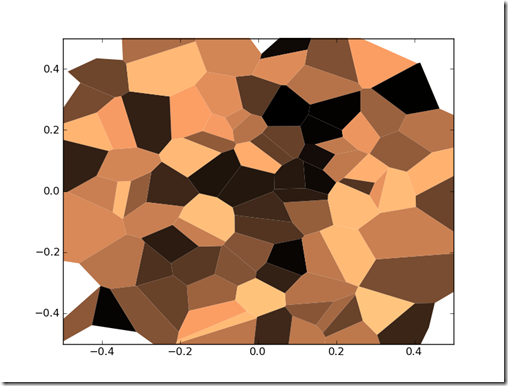
    result_list = voronoi2D(xpt,ypt,cpt,cmap=pp.cm.copper)
    
    pp.figure()
    for item in result_list:
        x_list = item[0]
        y_list = item[1]
        this_color = item[2]
        pp.fill(x_list,y_list,color=this_color,edgecolor='none')
    
   
    pp.axis([-0.5,0.5,-0.5,0.5])

    pp.show()


This work is licensed under a Creative Commons Attribution By license.

Sunday, March 20, 2011

Using Mathjax CDN to Embed Equations (Formulas) in a Web Page

$$ \begin{aligned} \nabla \times \vec{\mathbf{B}} -\, \frac1c\, \frac{\partial\vec{\mathbf{E}}}{\partial t} & = \frac{4\pi}{c}\vec{\mathbf{j}} \\ \nabla \cdot \vec{\mathbf{E}} & = 4 \pi \rho \\ \nabla \times \vec{\mathbf{E}}\, +\, \frac1c\, \frac{\partial\vec{\mathbf{B}}}{\partial t} & = \vec{\mathbf{0}} \\ \nabla \cdot \vec{\mathbf{B}} & = 0 \end{aligned} $$

Summary

Using Mathjax Content Delivery Network (CDN) equations and formulas can be added to a webpage with a few simple steps. This solution eliminates the need to setup and maintain a server. It is freely available for low bandwidth users. For some work flows, a document can be created offline and uploaded with little or no modification. This article summaries how to setup a webpage for use with Mathjax. The article provides a few examples of use.

Discussion

If you want to include equations in a blog, there are a few basic approaches. The simplest is to create pictures of the equations and embed those pictures in the web page. If you use MS Word to create HTML pages, this is how it embeds equations. Most of the standard options in Lyx for exporting to HTML use the same technique.  Alternatively, you can use some approach to render the equations at display time. The Google Chart API works like this. An image is embedded in a web page and the URL for the image contains a definition of the equation to display. Elyxer is a tool which converts a document written in Lyx into an HTML document which uses MathJax, jsMath, Google Chart API, or plain HTML to display the equations. This article shows how to manually use MathJax with a webpage.

Step 1: Add the MathJax scripts to the webpage.

You accomplish the first step by putting something like

<script type="text/javascript"
  src="http://cdn.mathjax.org/mathjax/latest/MathJax.js?config=TeX-AMS-MML_HTMLorMML">
</script>

into the <head> block of your document. This statement can be place in other locations like the <body>, but the <head> block is preferred. Since MathJax can be customized in many ways, there are many different ways to link MathJax to the webpage. The sample above works, but other configurations are possible. See the getting started guide for a detailed description of some of the options.

Step 2: Write your equations inside escape character sequences.

To add an equation, an escape sequence is entered. There is one escape sequence for inline equations and another for equations which appear on a line by themselves. For example, using the scrip method above, the sequence

$$…$$
and
\[ …\]
indicates that an equation is to appear by itself. The sequence
\(…\)

indicate that an equation should appear inline.

Below is a sample HTML page which includes MathJax.

<html>
  <head>
    <script type="text/javascript" src="/MathJax/MathJax.js?config=TeX-AMS-MML_HTMLorMML"></script>
  </head>
  <body>
    <p> Acceleration, \(a\), is a function of force, \(F\), and mass, \(m\). The relationship is usually written as \[F=m\cdot a\].<\p> However, by manipulating the equation, acceleration can be solved for as shown in equation (1).</p>
    <table border="0" cellspacing="0" cellpadding="2" width="100%">
      <tbody><
        <tr>
        <td valign="top" width="10%"></td>
        <td valign="top" width="80%"><p align="center">$$a=\frac{f}{m}$$</p></td>
        <td valign="top" width="10%">(1)</td>
        </tr>
    </tbody>
    </table>
  </body>
</html>


This code will result in a display like shown below:


Acceleration, \(a\), is a function of force, \(F\), and mass, \(m\). The relationship is usually written as \[F=m\cdot a\]. However, by manipulating the equation, acceleration can be solved for as shown in equation (1).


$$a=\frac{f}{m}$$

(1)


Conclusion

Thanks to the MathJax team and their sponsors. This is a fantastic service that really simplifies the maintenance and upkeep required to add equations to almost anything.


References:

This work is licensed under a Creative Commons Attribution By license.

Notes on installing a 2nd wireless router

image

Problem Statement

Given a 2wire 2701HG-B DSL modem with wireless router connected to the AT&T network and a Netgear N600 Dualband Router WNDR3400. The goal is to connect the two routers into a single network. All machines that are configured to work with the 2wire model should still work once the installation is complete. Ideally, no changes are required to the installed settings in the 2wire router. Both routers should behave like a single network, so regardless of where a device or computer connects, it can see all other devices on the local network. All devices should be able to see the internet regardless of where they connect.

Discussion

WARNING: I am not an network engineer. This discussion and the advice may have issues which result in network security performance issues. This configuration works to the extent it was tested. Use the advice with discretion.

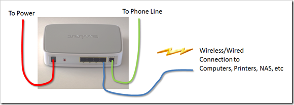
The initial installation consisted of a 2wire 2701HG-B DSL modem with wireless router. This was configured per AT&T instructions using the out-of-the-box installation software. This provided a wireless access point for the internet and local area network capable of about 50Mbps with 4 hard wired access points. The network initially supported b/g wireless connections. Several devices in the home were connected to the network. The setup panels for the 2wire gateway are accessible from  http://gateway.2wire.net .

Original Network and Gateway Configuration
image


A Netgear N600 Dualband Router, model WNDR3400 was obtained for faster local area network access. It supports a/b/g/n wireless access and had two channels so it can devices can connect to either the a/n channel on 5GHz or the b/g/n channel on 2.4 GHz.  In an optimal setting, both channels should be capable of 300Mbs. This router also has a USB port which can be configured as network storage: a drive which can be mapped in for use by any device on the network.

There was a fair amount of advice available on how to configure a second router. The key decision is on how the 2nd router should behave. One configuration is to establish a subnet. The 2nd router creates its own local area network which is isolated from the primary router. By opening firewall protections in the 2nd router, misc services like printing and device discover is possible between the primary local area network and the secondary local area network. The key disadvantage to this approach is that if you reconfigure the network in the future, the 2nd router has so many configuration changes it can be difficult to get the network working as expected. Another configuration is to have one router act as a master for the network and services in the other router partially disabled. This is necessary because each router is configured by default to do tasks which will conflict if they are connected together. Specifically, the DHCP services, which assign network addresses to connected devices, can only be performed by one router. So the DHCP services in the second router are disabled so only one router is assigning network addresses.

One last thing is that most routers are themselves devices which require an IP address. So if the second router shares a local area with another router, the IP addresses need to properly configures outside of any automatic address assignments.

The solution works through three network configurations. The first configuration allows devices connected to the second router to see the internet, but the two independent networks exist: devices can only see devices which are connected to the same local area network (LAN). The second configuration partially disables the firewall in the N600. This enables some printers on the primary LAN to be used by devices on the secondary LAN. Finally, both routers are connected together to form a single LAN and all devices can see each other regardless of which router they access.

Solution

Step 1: Configure the N600

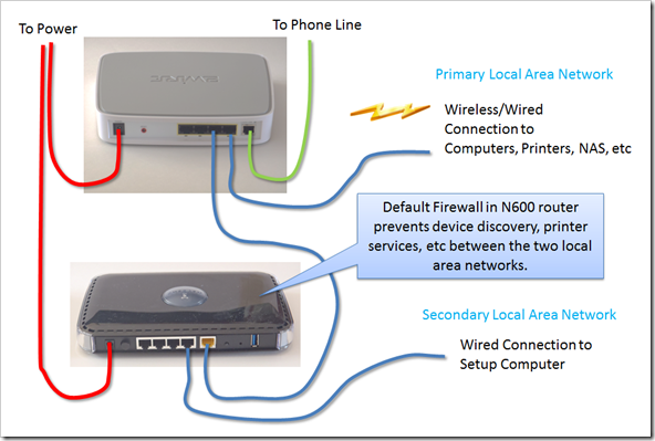
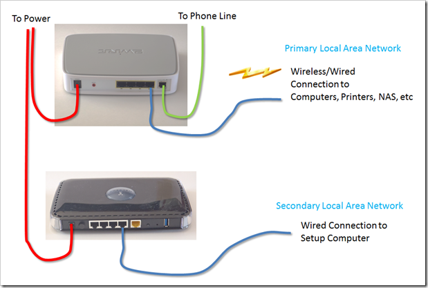
The first step in setting up the network is to install the N600 and configure it. The image below shows how the N600 is wired to the 2wire router. Once this is completed, the computer connected to the N600 is used to configure the N600 using the software disc which was provided. When this is complete, any device connected to the N600 should be able to see the internet through the 2wire gateway. If there is a problem, verify that the internet can be seen by connecting a device to the 2wire gateway. At this step, things like the wireless configuration for the N600 and wireless security can be configured.

Network Setup to configure N600 Router
image

In this configuration, each router assigned IP addresses to the components which connect to it. The firewall in the N600 prevents services like device discovery and printing from working across the network.

At this point, a device connected to the N600 can access the router configurations by connecting to http://www.routerlogin.net. This will bring up the administration page. It can be a good idea to change the admin password to prevent unwanted network changes.

Step 2: Disable NAT Filtering (optional).

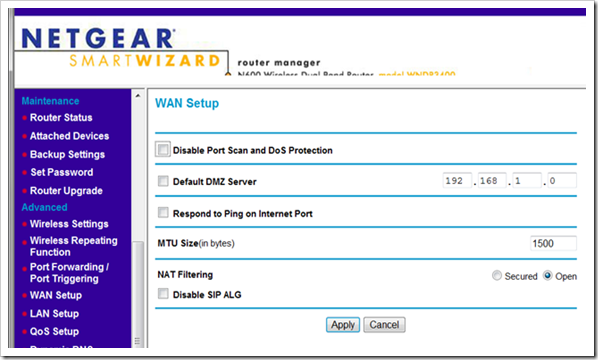
With a device connected to the N600, log into the administration pages at http://www.routerlogin.net. On the left had side of the screen, select ‘WAN Setup’. This let you modify what the N600 allows to pass between the two LANs. On the page that appears, set ‘NAT Filtering’ to ‘Open’. Click ‘Apply’ to save the change.
image

With this change, it should now be possible to access the internet and print to devices connected to the 2wire gateway from devices which are connected to the N600. This configuration can be useable and has a few advantages for situations where high traffic might be present. There are basically two independent networks and the only sharing between them is internet traffic.

Additional changes can probably configure the LAN on the N600 to allow devices on both LANs to see each other, but the testing for that was not done.

Step 3: Reconfigure N600 to share same LAN

This step requires a few things to be done before any testing can be done to confirm the job was done correctly. So there are a few places where things can go wrong.

Step 3a: Identify where the 2wire gateway assigns addresses.

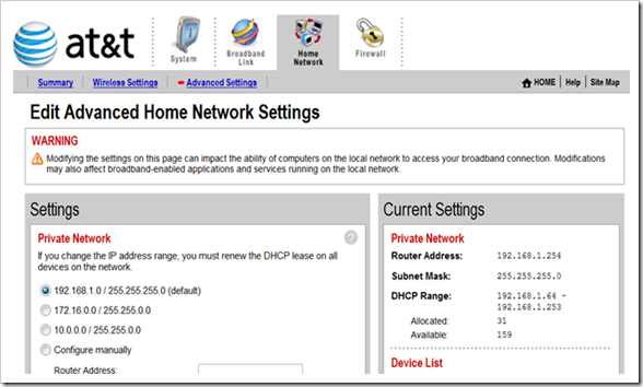
With a device connected to the 2wire gateway, log into http://gateway.2wire.net. Select ‘Home Networking’ and ‘Advanced Settings’. The ‘Private Network’ panel should show where the 2wire gateway assigns IP addresses. In the example below, the base address is 192.168.1.0. By looking at the ‘Current Settings’ the range of assigned addresses can be seen. In this case, the range of assigned addresses are 192.168.1.64 through 192.168.1.253. Keep this range in mind.
image

Step 3b: Disconnect the N600 from the 2Wire gateway.
image

Step 3c: Reconfigure the N600.

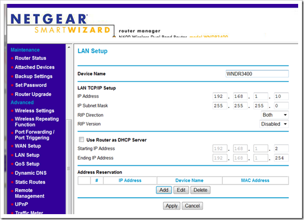
To reconfigure the N600, the DHCP services will be turned off and the IP address of the N600 will be set in address range of the 2wire gateway but outside of the DHCP range for the 2wire gateway. For this system, an address of 192.168.1.10 will work.

With a computer connected to the N600, connect to http://www.routerlogin.net and go to the LAN Setup page. On that page enter 192.168.1.10 as the IP address and unselect ‘Use Router as DHCP Server’. This sets up the address the N600 will appear at in the future and prevents the N600 from assigning network addresses.  Click ‘Apply’. The N600 will reset and you may lose communication because the network addresses will no longer be valid. If this happens everything is fine. However you will not be able to do anything with this setup until you do the next step.
image

Step 3d: Reconnect the N600 to the 2wire.

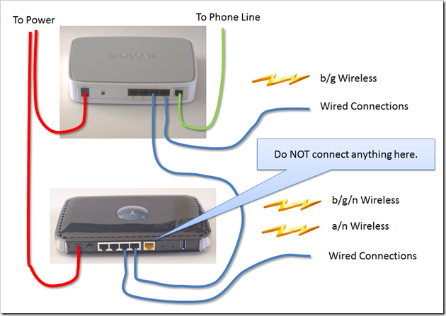
Connect one of the LAN ports on the N600 to a LAN port on the 2wire. Do NOT connect anything to the WAN port of the N600. Do NOT use a cross-over cable (If you do not know what this is, do not worry about it).
image

Step 4: Testing

To test this system, connect a device to the N600. Try to log into the 2wire at http://gateway.2wire.net. If the setup is working, you should be able to log into the 2wire gateway. This proves the N600 and the 2wire are sharing the same LAN. Next log into the N600. Unfortunately, the convenient login address will no longer work since the DHCP services in the N600 were disables. So you have to log in using the IP address: http://192.168.1.10. If you can do this, chances are things are now correctly configured.

Conclusion:

You should have 6 wired ports available (3 on the 2wire, 3 on the N600) and 3 wireless connection options: a b/g wireless connection on the 2wire, a b/g/n connection on the N600, and an a/n connection on the N600.  All devices on these connects should be able to see each other and the internet.
This work is licensed under a Creative Commons Attribution By license.

Saturday, March 19, 2011

MathJax Test Posting

This is a test to confirm that MathJax works.

When \(a \ne 0\), there are two solutions to \(ax^2 + bx + c = 0\) and they are
$$x = {-b \pm \sqrt{b^2-4ac} \over 2a}.$$

Thursday, March 10, 2011

A Python Script to Fit an Ellipse to Noisy Data

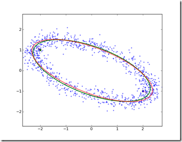
ExampleEllipse

Problem statement

Given a set of noisy data which represents noisy samples from the perimeter of an ellipse, estimate the parameters which describe the underlying ellipse.

Discussion

There are two general ways to fit an ellipse: algebraic and geometric approaches. In an algebraic approach, the parameters for an algebraic description of an ellipse are fit subject to constraints which guarantee the parameters result in an ellipse. In the geometric approach,  characteristics of the ellipse are fit.

The code snippet below uses a method described by Yu, Kulkarni & Poor. The location of the foci and the length of the line segments from the foci to a point on the perimeter of the ellipse are found through an optimization problem. Because the fitting objective is not convex and has a minimum at infinity, a penalty cost is added to prevent the foci from wandering off.

Code

'''
Script to fit an ellipse to a set of points.
- The ellipse is represented by the two foci and the length of a 
     line segment which is drawn from the foci to the 
     point where the ellipse intersects the minor axis.
    
- Fitting algorithm from Yu, Kulkarni & Poor

'''

__author__ = 'Ed Tate'
__email__  = 'edtategmail-dot-com'
__website__ = 'exnumerus.blogspot.com'
__license__ = 'Creative Commons Attribute By - http://creativecommons.org/licenses/by/3.0/us/'''

####################################################
# create ellipse with random noise in points
from random import uniform,normalvariate
from math import pi, sin, cos, exp, pi, sqrt
from openopt import NLP
from numpy import *
from numpy import linalg as LA
import matplotlib.pylab as pp

def gen_ellipse_pts(a,foci1,foci2,
                    num_pts=200, angles=None,
                    x_noise = None, y_noise=None):

    '''
       Generate points for an ellipse given
          the foci, and
          the distance to the intersection of the minor axis and ellipse.
    
       Optionally, 
          the number of points can be specified,
          the angles for the points wrt to the centroid of the ellipse, and 
          a noise offset for each point in the x and y axis.
    '''
    c = (1/2.0)*LA.norm(foci1-foci2)
    b = sqrt(a**2-c**2)
    x1 = foci1[0]
    y1 = foci1[1]
    x2 = foci2[0]
    y2 = foci2[1]
    if angles is None:
        t = arange(0,2*pi,2*pi/float(num_pts))
    else:
        t = array(angles)
            
    ellipse_x = (x1+x2)/2 +(x2-x1)/(2*c)*a*cos(t) - (y2-y1)/(2*c)*b*sin(t)
    ellipse_y = (y1+y2)/2 +(y2-y1)/(2*c)*a*cos(t) + (x2-x1)/(2*c)*b*sin(t)
    try:
        # try adding noise to the ellipse points
        ellipse_x = ellipse_x + x_noise
        ellipse_y = ellipse_y + y_noise
    except TypeError:
        pass
    return (ellipse_x,ellipse_y)

####################################################################

# setup the reference ellipse

# define the foci locations
foci1_ref = array([2,-1])
foci2_ref = array([-2,1])
# pick distance from foci to ellipse
a_ref = 2.5

# generate points for reference ellipse without noise
ref_ellipse_x,ref_ellipse_y = gen_ellipse_pts(a_ref,foci1_ref,foci2_ref)

# generate list of noisy samples on the ellipse
num_samples = 1000
angles = [uniform(-pi,pi) for i in range(0,num_samples)]
sigma = 0.2
x_noise = [normalvariate(0,sigma) for t in angles]
y_noise = [normalvariate(0,sigma) for t in angles]
x_list,y_list = gen_ellipse_pts(a_ref,foci1_ref,foci2_ref,
                                angles  = angles,
                                x_noise = x_noise,
                                y_noise = y_noise)

point_list = []
for x,y in zip(x_list,y_list):
    point_list.append(array([x,y]))    

# draw the reference ellipse and the noisy samples    
pp.figure()
pp.plot(x_list,y_list,'.b', alpha=0.5)
pp.plot(ref_ellipse_x,ref_ellipse_y,'g',lw=2)
pp.plot(foci1_ref[0],foci1_ref[1],'o')
pp.plot(foci2_ref[0],foci2_ref[1],'o')

#####################################################

def initialize():
    '''
    Determine the initial value for the optimization problem.
    '''
    # find x mean
    x_mean = array(x_list).mean()
    # find y mean
    y_mean = array(y_list).mean()
    # find point farthest away from mean
    points = array(zip(x_list,y_list))
    center = array([x_mean,y_mean])
    distances = zeros((len(x_list),1))
    for i,point in enumerate(points):
        distances[i,0]=LA.norm(point-center)
    ind = where(distances==distances.max())
    max_pt = points[ind[0],:][0]
    # find point between mean and max point
    foci1 = (max_pt+center)/2.0
    # find point opposite from 
    foci2 = 2*center - max_pt
    return [distances.max(), foci1[0],foci1[1],foci2[0],foci2[1]]


def objective(x):
    '''
    Calculate the objective cost in the optimization problem.
    '''
    foci1 = array([x[1],x[2]])
    foci2 = array([x[3],x[4]])
    a     = x[0]
    n = float(len(point_list))
    _lambda =0.1
    _sigma = sigma
    sum = 0
    for point in point_list:
        sum += ((LA.norm(point-foci1,2)+LA.norm(point-foci2,2)-2*a)**2)/n
    sum += _lambda*ahat_max*_sigma*exp((a/ahat_max)**4)
    return sum

# solve the optimization problem
x0 = initialize()
ahat_max = x0[0]
print x0
p = NLP(objective, x0)
r = p.solve('ralg')
print r.xf

# get the results from the optimization problem
xf = r.xf
# unload the specific values from the result vector
foci1 = array([xf[1],xf[2]])
foci2 = array([xf[3],xf[4]])
a     = xf[0]

# reverse the order of the foci to get closest to ref foci
if LA.norm(foci1-foci1_ref)>LA.norm(foci1-foci2_ref):
    _temp = foci1
    foci1 = foci2
    foci2 = _temp

####################################################
# plot the fitted ellipse foci
pp.plot([foci1[0]],[foci1[1]],'xk')
pp.plot([foci2[0]],[foci2[1]],'xk')

# plot a line between the fitted ellipse foci and the reference foci
pp.plot([foci1[0],foci1_ref[0]],[foci1[1],foci1_ref[1]],'m-')
pp.plot([foci2[0],foci2_ref[0]],[foci2[1],foci2_ref[1]],'m-')

# plot fitted ellipse
(ellipse_x,ellipse_y) = gen_ellipse_pts(a,foci1,foci2,num_pts=1000)  
pp.plot(ellipse_x,ellipse_y,'r-',lw=3,alpha=0.5)

# scale the axes for a square display
x_max = max(x_list)
x_min = min(x_list)
y_max = max(y_list)
y_min = min(y_list)

box_max = max([x_max,y_max])
box_min = min([x_min,y_min])
pp.axis([box_min, box_max, box_min, box_max])

pp.show()


References


Testing Configuration

This work is licensed under a Creative Commons Attribution By license.

Tuesday, March 8, 2011

A Python Recipe to Interactively Identify Elements in Matplotlib

Problem Statement

You need to interactively identify a point in a Matplotlib plot.

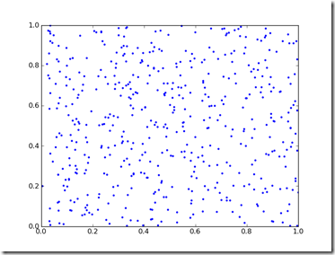
example_plot

Solution

This solution requires three parts. First, a function is defined which is executed when a plot element is selected. Second, this function is connected to the figure. Finally, when a point is plotted, a picker radius is added which defines how big of an area should react to the pick event. One way to get a unique response from each point is to add an attribute to each point. In this example, a string is added with information about the point location. More complex responses can be created by considering an attribute like this in ‘onpick’ function.

__author__ = 'Ed Tate'
__email__  = 'edtate<at>gmail-dot-com'
__website__ = 'exnumerus.blogspot.com'
__license__ = 'Creative Commons Attribute By - http://creativecommons.org/licenses/by/3.0/us/'''

import matplotlib.pylab as p
import random

# define what should happen when a point is picked
def onpick(event):
    thisline = event.artist
    name = thisline.name
    print name

# create the figure and add the handler which reacts to a pick event
fig = p.figure()
fig.canvas.mpl_connect('pick_event',onpick)

# create random set of points to plot
x_pts = [random.uniform(0,1) for i in range(0,500)]
y_pts = [random.uniform(0,1) for i in range(0,500)]

for x,y in zip(x_pts,y_pts):
    pt, = p.plot(x,y,'.b',picker=3)
    pt.name = 'Point located at (%f,%f)' % (x,y)
    

p.show()

When this script is executed, picking a point results in a message which shows which point was chosen:

Point located at (0.481866,0.661643)


References


Testing Conditions

This work is licensed under a Creative Commons Attribution By license.

Tuesday, March 1, 2011

Rough Draft: How to generate 2D Delaunay Triangulations using Qhull and Python

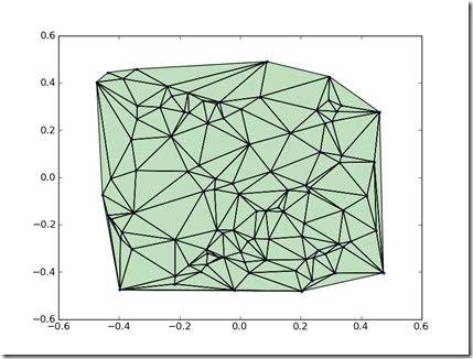
Delaunay triangulations partition a space into regions. Delaunay triangulations can be useful for interpolation and visualizing spatial data.

sample_delaunay

Qhull is a program which can generate tesselations, convex hulls, and vonoroi diagrams from a set of points. This program is available as a precompiled executable and source code. By interfacing to the command line version of this program, a Delaunay triangulation can be generated.

Sample CodE

To use this code, download Qhull and copy the ‘qhull.exe’ to the working directory. Make sure the code has read, write, and execute privileges in the working directory. Make sure there are not files named ‘data.txt’ or ‘results.txt’ which need to be preserved.

'''
This module generates 2D tesselations for a set of points.
The vornoi cells can be filtered by supplying a value associated with 
   each node.
'''

__author__ = 'Ed Tate'
__email__  = 'edtate-at-gmail-dot-com'

def delaunay2D(xpt,ypt,cpt=None,threshold=0):
    
    if cpt is None:
        cpt = [-1 for x in xpt]    
        
    # write the data file
    pts_filename = 'data.txt'
    pts_F = open(pts_filename,'w')
    #print pts_F
    pts_F.write('2 # this is a 2-D input set\n')
    pts_F.write('%i # number of points\n' % len(xpt))
    for i,(x,y) in enumerate(zip(xpt,ypt)):
        pts_F.write('%f %f # data point %i\n' % (x,y,i))
    pts_F.close()

    # trigger the shell command
    import subprocess

    p = subprocess.Popen('qhull TI data.txt TO results.txt d i Qc Qt Qbb', shell=True)
    p.wait()

    # open the results file and parse results
    results = open('results.txt','r')
    print results

    # get 'i' results
    data = results.readline()
    tri_list = []
    numLines = int(data)
    print numLines
    for i in range(numLines):
        # load each triplet of indexes to x,y points
        data = results.readline()
        idx1,idx2,idx3,dummy = data.split(' ')
        idx1 = int(idx1)
        idx2 = int(idx2)
        idx3 = int(idx3)
        tri_list.append([idx1,idx2,idx3])
        
    #################
    #this generates a fillable collection of tesselations
    x_list = []
    y_list = []   
    
    for t in tri_list:
        if all([ cpt[t[i]]<threshold for i in range(3)]):
            short_x_list = [ xpt[t[i]] for i in range(3)]
            short_y_list = [ ypt[t[i]] for i in range(3)]
            x_list.extend(short_x_list)
            x_list.append(xpt[t[0]])
            x_list.append(None)
            y_list.extend(short_y_list)
            y_list.append(ypt[t[0]])
            y_list.append(None)
    
    return (x_list,y_list)


if __name__=='__main__':
    
    import random
    
    N=100
    xpt = [random.random()-0.5 for i in range(0,N)]
    ypt = [random.random()-0.5 for i in range(0,N)]
    cpt = [random.random()-0.5 for i in range(0,N)]
    
    import matplotlib.pyplot as pp
    
    pp.figure()
    (x_list,y_list) = delaunay2D(xpt,ypt,cpt)
    pp.plot(xpt,ypt,'b.')
    pp.plot(x_list,y_list,'k-')

    pp.fill(x_list,y_list,'g',alpha=0.25,edgecolor='none')    

    pp.show()
    

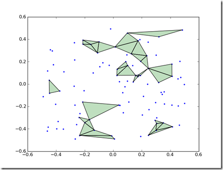
When run, this module will produce a diagram with the cells with filled triangulation where the vertices have a random value greater than 0.

sample_delaunay_2

Test Conditions


Answers

  • How to tesselate a set of points
  • How to generate a Delaunay Triangulation
  • How to use Qhull with Python
This work is licensed under a Creative Commons Attribution By license.