Sunday, February 27, 2011

Rough Draft: How to Generate Voronoi Diagrams in Python & Matplotlib

Voronoi diagrams partition a space into cells. Each cell represents the region nearest a point  in a set. Voronoi diagrams can be useful for visualizing spatial data.

sample_voronoi

Qhull is a program which can generate tesselations, convex hulls, and vonoroi diagrams from a set of points. This program is available as a precompiled executable and source code. By interfacing to the command line version of this program, a Voronoi diagram can be generated in Matplotlib.

Sample CodE

To use this code, download Qhull and copy the ‘qvoronoi.exe’ to the working directory. Make sure the code has read, write, and execute privileges in the working directory. Make sure there are not files named ‘data.txt’ or ‘results.txt’ which need to be preserved.

'''
This module generates 2D voronoi diagrams from a list of points.
The vornoi cells can be filtered by supplying a value associated with 
   each node.
'''

def voronoi2D(xpt,ypt,cpt=None,threshold=0):
    '''
    This function returns a list of line segments which describe the voronoi
        cells formed by the points in zip(xpt,ypt).
    
    If cpt is provided, it identifies which cells should be returned.
        The boundary of the cell about (xpt[i],ypt[i]) is returned 
            if cpt[i]<=threshold.
            
    This function requires qvoronoi.exe in the working directory. 
    The working directory must have permissions for read and write access.
    This function will leave 2 files in the working directory:
        data.txt
        results.txt
    This function will overwrite these files if they already exist.
    '''
    
    if cpt is None:
        # assign a value to cpt for later use
        cpt = [0 for x in xpt]
    
    # write the data file
    pts_filename = 'data.txt'
    pts_F = open(pts_filename,'w')
    pts_F.write('2 # this is a 2-D input set\n')
    pts_F.write('%i # number of points\n' % len(xpt))
    for i,(x,y) in enumerate(zip(xpt,ypt)):
        pts_F.write('%f %f # data point %i\n' % (x,y,i))
    pts_F.close()

    # trigger the shell command
    import subprocess
    p = subprocess.Popen('qvoronoi TI data.txt TO results.txt p FN Fv QJ', shell=True)
    p.wait()

    # open the results file and parse results
    results = open('results.txt','r')

    # get 'p' results - the vertices of the voronoi diagram
    data = results.readline()
    voronoi_x_list = []
    voronoi_y_list = []
    data = results.readline()
    for i in range(0,int(data)):
        data = results.readline()
        xx,yy,dummy = data.split(' ')    
        voronoi_x_list.append(float(xx))
        voronoi_y_list.append(float(yy))
        
    # get 'FN' results - the voronoi edges
    data = results.readline()
    voronoi_idx_list = []
    for i in range(0,int(data)):
        data = results.readline()
        this_list = data.split(' ')[:-1]
        for j in range(len(this_list)):
            this_list[j]=int(this_list[j])-1
        voronoi_idx_list.append(this_list[1:])
        
    # get 'FV' results - pairs of points which define a voronoi edge
    # combine these results to build a complete representation of the 
    data = results.readline()
    voronoi_dict = {}
    for i in range(0,int(data)):
        data = results.readline().split(' ')

        pair_idx_1 = int(data[1])
        pair_idx_2 = int(data[2])

        vertex_idx_1 = int(data[3])-1
        vertex_idx_2 = int(data[4])-1

        try:
            voronoi_dict[pair_idx_1].append({ 'edge_vertices':[vertex_idx_1,vertex_idx_2],
                                      'neighbor': pair_idx_2 })
        except KeyError:
            voronoi_dict[pair_idx_1] = [{ 'edge_vertices':[vertex_idx_1,vertex_idx_2],
                                      'neighbor': pair_idx_2 } ]

        try:
            voronoi_dict[pair_idx_2].append({ 'edge_vertices':[vertex_idx_1,vertex_idx_2],
                                      'neighbor': pair_idx_1 })
        except KeyError:
            voronoi_dict[pair_idx_2] = [{ 'edge_vertices':[vertex_idx_1,vertex_idx_2],
                                      'neighbor': pair_idx_1 } ]    

                    
    #################
    # generate a collection of voronoi cells
    x_list = []
    y_list = []    
    for point_idx in voronoi_dict.keys():
        if cpt[point_idx]<=threshold:
            # display this cell, so add the data to the edge list
            e_list = []
            for edge in voronoi_dict[point_idx]:
                p1_idx = edge['edge_vertices'][0]
                p2_idx = edge['edge_vertices'][1]
                e_list.append((p1_idx,p2_idx))
            
            # put the vertices points in order so they
            #   walk around the voronoi cells
            p_list = [p1_idx]
            while True:
                p=p_list[-1]
                for e in e_list:
                    if p==e[0]:
                        next_p = e[1]
                        break
                    elif p==e[1]:
                        next_p = e[0]
                        break
                p_list.append(next_p)
                e_list.remove(e)
                if p_list[0]==p_list[-1]:
                    # the cell is closed
                    break
                
            # build point list
            if all([p>=0 for p in p_list]):
                for p in p_list:
                    if p>=0:
                        x_list.append(voronoi_x_list[p])
                        y_list.append(voronoi_y_list[p])                    
            x_list.append(None)
            y_list.append(None)
                    
    return (x_list,y_list)

if __name__=='__main__':
    
    import random
    
    xpt = [random.random()-0.5 for i in range(0,100)]
    ypt = [random.random()-0.5 for i in range(0,100)]
    cpt = [random.random()-0.5 for i in range(0,100)]
    
    (x_list,y_list) = voronoi2D(xpt,ypt,cpt)
    
    import matplotlib.pyplot as pp
    
    pp.figure()
    pp.plot(xpt,ypt,'b.')
    pp.plot(x_list,y_list,'k-')
    
    pp.fill(x_list,y_list,'g',alpha=0.25,edgecolor='none')    
     
    pp.axis([-1,1,-1,1])

    pp.show()


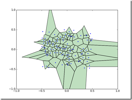
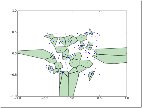
When run, this module will produce a Voronoi diagram with the cells which have a value greater than zero visible.
sample_voronoi_2

Test Conditions

This work is licensed under a Creative Commons Attribution By license.

How to quickly plot polygons in Matplotlib

Problem statement:

You need to plot a large collection of polygons in Matplotlib.

Solution:

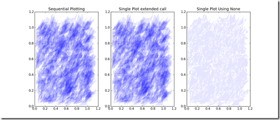
A simple way to plot filled polygons in Matplotlib is to use the fill function. If you try to plot a collection of  polygons in Matplotlib using sequential calls to fill, it can take a lot of time to generate the graph. There are two ways to speed up the plotting. The first is to use Python’s extended call syntax and pass multiple polygons at one time. The other is to create a single list of points which are the corners of the polygon and separate each polygon by a ‘None’ entry. The extended call method yields an appreciable improvement in performance. Forming a single list of polygon corners separated by ‘None’ results in a significant time savings. For the test cases below, using extended call syntax decreased drawing time by about 50% and using a single list separated by ‘None’ decreased drawing time by about 99%.

Execution time for sequential plotting = 2.496564 sec
Execution time for extended call plotting = 1.172675 sec  
Execution time when using None = = 0.028234 sec

Sample Code:

'''
Code snippet to plot multiple triangle's in Matplotlib using different methods.
'''
import time
import sys
import matplotlib.pyplot as pp
import random

if sys.platform == "win32":
     # On Windows, the best timer is time.clock()
     default_timer = time.clock 
else:     
    # On most other platforms the best timer is time.time()     
    default_timer = time.time
    
    
# generate ends for the triangle line segments
xtris = []
ytris = []
for i in range(1000):
    x1 = random.random()
    x2 = x1 + random.random()/5.0
    x3 = x1 + random.random()/5.0
    xtips = [x1,x2,x3]
    y1 = random.random()
    y2 = y1 + random.random()/5.0
    y3 = y1 + random.random()/5.0
    ytips = [y1,y2,y3]
    xtris.append(xtips)
    ytris.append(ytips)

############################
# time sequential call to matplotlib
pp.figure()
pp.subplot(1,3,1)

t0 = default_timer()
for xtips,ytips in zip(xtris,ytris):
    pp.fill(xtips,ytips,
            facecolor='b',alpha=0.1, edgecolor='none')
t1 = default_timer()

pp.title('Sequential Plotting')

print 'Execution time for sequential plotting = %f sec' % (t1-t0)

# rebuild ends using none to separate polygons
xlist = []
ylist = []
for xtips,ytips in zip(xtris,ytris):
    xlist.extend(xtips)
    xlist.append(None)
    ylist.extend(ytips)
    ylist.append(None)

############################
# build argument list
call_list = []
for xtips,ytips in zip(xtris,ytris):
    call_list.append(xtips)
    call_list.append(ytips)
    call_list.append('-b')
    
############################
# time single call to matplotlib
pp.subplot(1,3,2)

t0 = default_timer()
pp.fill(*call_list,
            facecolor='b',alpha=0.1, edgecolor='none')

t1 = default_timer()

pp.title('Single Plot extended call')

print 'Execution time for extended call plotting = %f sec' % (t1-t0)

    
############################
# time single call to matplotlib
pp.subplot(1,3,3)

t0 = default_timer()
pp.fill(xlist,ylist,
        facecolor='b',alpha=0.1,edgecolor='none')
t1 = default_timer()

pp.title('Single Plot Using None')

print 'Execution time when using None = %f sec' % (t1-t0)

pp.show()

Discussion:

   Sequential call and extended call syntax produce the same plot results. However, the single list of points using ‘None’ can generate a different image if transparency is used. In the sample code, ‘alpha=0.1’ was used. When sequential fill or extended call syntax is used, the color from each polygon is additive. When the polygon corners are combined into a single list of points, the polygon colors are not additive. This is only an issue when using transparency. If alpha is set to 1.0 (or not set at all), then all of the plots will be identical.

PolygonSample


Test Conditions:


Answers:

  • How to speed up Matplotlib plots
  • How to plot polygons in Matplotlib
This work is licensed under a Creative Commons Attribution By license.

How to quickly plot multiple line segments in Matplotlib

Problem statement:

You need to plot a large collection of line segments in Matplotlib.

Solution:

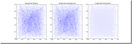
If you try to plot a collection of  lines segments in Matplotlib using sequential calls to plot, it can take a lot of time to generate the graph. There are two ways to speed up the plotting. The first is to use pythons extended call syntax and pass multiple lines segments at a time. The other is to create a single list of points, where the line segments are separated by ‘None’ values. The extended call method yields a minor improvement in performance. Forming a single list of line segments separated by ‘None’ results in a significant time savings. For the test cases below, using extended call syntax decreased drawing time by about 10% and using a single list separated by ‘None’ decreased drawing time by more than 99%.

Execution time for sequential plotting = 11.083103 sec
Execution time for extended call plotting = 10.245883 sec
Execution time when using None = = 0.027801 sec

Sample Code:

import time
import sys
import matplotlib.pyplot as pp
import random

if sys.platform == "win32":
     # On Windows, the best timer is time.clock()
     default_timer = time.clock 
else:     
    # On most other platforms the best timer is time.time()     
    default_timer = time.time
    
    
# generate ends for the line segments
xpairs = []
ypairs = []
for i in range(1000):
    xends = [random.random(), random.random()]
    yends = [random.random(), random.random()]
    xpairs.append(xends)
    ypairs.append(yends)

############################
# time sequential call to matplotlib
pp.figure()
pp.subplot(1,3,1)

t0 = default_timer()
for xends,yends in zip(xpairs,ypairs):
    pp.plot(xends,yends,'b-',alpha=0.1)
t1 = default_timer()

pp.title('Sequential Plotting')

print 'Execution time for sequential plotting = %f sec' % (t1-t0)

############################
# build argument list
call_list = []
for xends,yends in zip(xpairs,ypairs):
    call_list.append(xends)
    call_list.append(yends)
    call_list.append('-b')
    
############################
# time single call to matplotlib
pp.subplot(1,3,2)

t0 = default_timer()
pp.plot(*call_list,alpha=0.1)
t1 = default_timer()

pp.title('Single Plot extended call')

print 'Execution time for extended call plotting = %f sec' % (t1-t0)

############################
# rebuild ends using none to separate line segments
xlist = []
ylist = []
for xends,yends in zip(xpairs,ypairs):
    xlist.extend(xends)
    xlist.append(None)
    ylist.extend(yends)
    ylist.append(None)
    
############################
# time single call to matplotlib
pp.subplot(1,3,3)

t0 = default_timer()
pp.plot(xlist,ylist,'b-',alpha=0.1)
t1 = default_timer()

pp.title('Single Plot Using None')

print 'Execution time when using None = %f sec' % (t1-t0)

pp.show()

Discussion:

   Sequential call and extended call syntax produce the same results. However, the single list of points using ‘None’ can generate a different image if transparency is used. In the sample code, ‘alpha=0.1’ was used. When sequential plots or extended call syntax is used, the color from each line segment is additive. When the line segments were combined into a single list of points, the line segments’ color was not additive. This is only an issue when using transparency. If alpha is set to 1.0 (or not set at all), then all of the plots will be identical.

ExamplePlot


Test Conditions:


Answers:

  • How to speed up Matplotlib plots
  • How to plot lines in Matplotlib
This work is licensed under a Creative Commons Attribution By license.