Weighted Curve Fitting.

Introduction
When using least-squares linear regression, an assumption in typical implementations is that the noise is Gaussian, white, and has the same statistics for all measurements. All of the solutions discussed in part 1 of this tutorial make this assumption including the polyfit function. This means that the regression will only work correctly is the measurement device always has the same statistics in its measurement errors. Sometimes, when data is collected, the noise statistics vary with each measurement. For example, this can happen when the background noise changes over time. Weighted least squares is a way to find fit a curve or find parameters when this occurs.
An Example

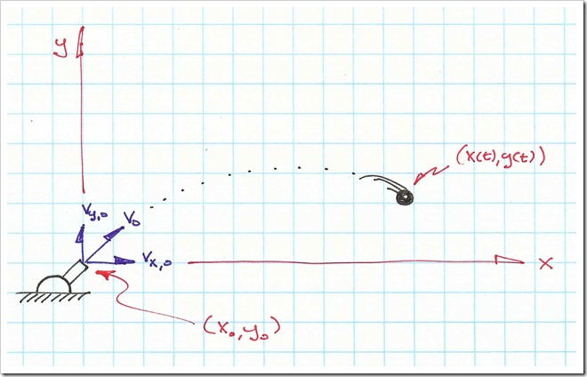
Consider a simplified ballistic problem. Ignoring the effect of air resistance, the vertical position of a projective is governed by its initial position, initial velocity, and the force of gravity. Since air resistance is not considered, the measured altitude of projectile is a closed form function of time:

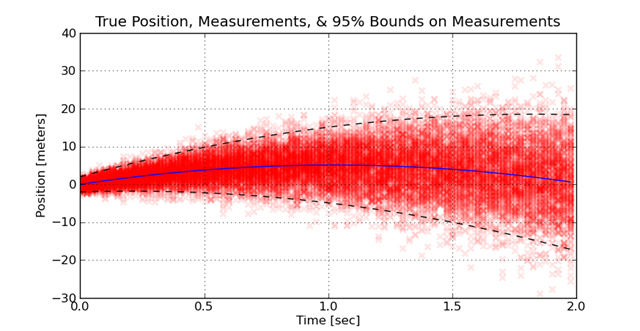
The noise term at the end of the equation is the error introduced by the measurement system. The noise, varies as a function of time and is represented by a normal distribution with time varying variance. For this problem, assume the noise gets worse with each subsequent sample. The mean of the error in each measurement is zero and has a standard deviation equal to 1 plus 4 times the number of seconds since the measurements started:

This might happen because the measurement hardware heats up with each sample, or the projectile moves away from the sensor. To visualize how this distribution of measurement errors looks, the measurements are taken many times. Each experiment is plotted over the previous experiments. The density of the measurements provides a visual feel for how the increase in error spreads out the measurements. This is illustrated here:
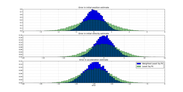
 The challenge in this kind of problem is using the knowledge of the model of the behavior (e.g. the ballistics) and the model of the noise to find an optimal fit. If a suboptimal method is used, the error in the fit is significantly greater than if an optimal method is used. A single comparison on a one data set is insufficient to see the benefits of one approach versus another. When a large number of experiments are performed where the true value is know and the estimated values are know, the distribution of the estimation errors due to different approaches is visible. The following graph shows how using weighted least-squares versus least-squares assuming constant weights improves on the distribution of errors.
 These graphs were generated from the following script:
from random import normalvariate
from pylab import *

class System(object):
    def __init__(self,p0=0.0,v0=10.0,a=-9.8):
        self.p0 = p0
        self.v0 = v0
        self.a = a

    def position(self,time):
        return self.p0+self.v0*t+0.5*self.a*t**2

class Sensor(object):
    def __init__(self,system=System(),errorStd=0.0):
        self.system = system
        self.errorStd = errorStd
    def error(self,t=0):
        try:
            std = self.errorStd(t=t)
            err = normalvariate(0,std)
        except TypeError:
            err = normalvariate(0,self.errorStd)
        return err

class PositionSensor(Sensor):
    def measure(self,t):
        err = Sensor.error(self,t=t)
        return self.system.position(t)+err

    def errorStd(self,t):
        try:
           return self.errStd(t)
        except TypeError:
            return self.errStd


def weightedPolyFit(xList,yList,sigmaList,order=1,crossesAtZero=False):
    '''fit the data using a weighted least squares for a polynomial model
        xList is a list of input values
        yList is a list of output values
        sigmaList is a list with the standard deviation for each y value
        order defines the order of the model,
            order = 1 -> linear model
            order = 2 -> quadratic model
        crossesAtZero specifies whether the polynomial must be equal to zer
            at x = 0
    '''
    fList = [(lambda x,n=n: x**n) for n in range(order,-1,-1)]
    if crossesAtZero:
        # eliminate the first column so the model corsses at 0
        del fList[0]
    # build row for each element in y
    bList = []
    A_List = []
    for (thisX,thisY) in zip(xList,yList):
        bList.append(thisY)
        A_Row = [f(thisX) for f in fList]
        A_List.append(A_Row)
    W = diag([1.0 /sigma for sigma in sigmaList])
    b = matrix(bList).T
    A = matrix(A_List)
    b2 = W*b
    A2 = W*A
    w = inv(A2.T*A2)*A2.T*b2
    return w.T.tolist()[0]


if __name__=='__main__':
    import random

    errStdFun = lambda t: 1 + 4.0*t

    random.seed(0)

    p0True = 0.0
    v0True = 10.0
    aTrue = 9.8

    s = System()
    p = PositionSensor(s,errStdFun)
    tSamples = arange(0,2,0.025)

    pErr1List = []
    pErr2List = []
    vErr1List = []
    vErr2List = []
    aErr1List = []
    aErr2List = []

    for i in range(0,20000):
        measuredPosition = [p.measure(t) for t in tSamples]

        xList = tSamples
        yListMeasured = measuredPosition
        sigmaList = [p.errorStd(t) for t in tSamples]
        w =  weightedPolyFit(xList,yListMeasured,sigmaList,order=2)
        p0Est = w[2]
        v0Est = w[1]
        aEst  = w[0]*2
        pErr1List.append(p0Est-p0True)
        vErr1List.append(v0Est-v0True)
        aErr1List.append(aEst-aTrue)

        w2 =  polyfit(xList,yListMeasured,2)
        p0Est2 = w2[2]
        v0Est2 = w2[1]
        aEst2  = w2[0]*2
        pErr2List.append(p0Est2-p0True)
        vErr2List.append(v0Est2-v0True)
        aErr2List.append(aEst2-aTrue)

    figure(1)
    subplot(3,1,1)
    hist(pErr1List,50,normed=True)
    hist(pErr2List,50,normed=True,alpha=0.5)
    grid(True)
    title('Error in initial position estimate')


    subplot(3,1,2)
    hist(vErr1List,50,normed=True)
    hist(vErr2List,50,normed=True,alpha=0.5)
    grid(True)
    title('Error in initial velocity estimate')

    subplot(3,1,3)
    hist(aErr1List,50,normed=True,label='Weighted Least Sq Fit')
    hist(aErr2List,50,normed=True,label='Least Sq Fit',alpha=0.5)
    legend()
    grid(True)
    xlabel('error')
    title('Error in acceleration estimate')


    show()
Some Theory: Finding the best fit
Recall from pt 1, that a least-squares fit is performed by reducing the equations to a matrix expression,
 then using the KKT conditions to find the weights which minimize the sum of errors squared.
In weighted least-squares, each error can have a different relative importance in the minimization problem. Usually, this weighting is equal to the inverse of the standard deviation of the error and each error is assumed to be uncorrelated. If these conditions are met, the relative weighting is in a diagonal matrix. Using the KKT conditions, this minimization problem,

is solved using

The solved example
To solve this problem, a system class and a sensor class is created. The sensor class is subclassed into a position sensor. The system class provides a model of the true behavior of the system. The sensor class provides a model of the data measured by a sensor which detecting the true position of the system in the presence of noise.
The weightedPolyFit function, in the listing, provides the logic to generate a weighted fit for parameters in a polynomial equation, which describes the position of the projectile.
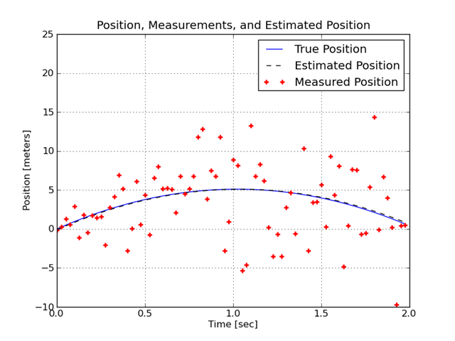
This plot shows the true trajectory of the projectile, the measured positions, and the estimated positions.

The full code for the example
from random import normalvariate
from pylab import *

class System(object):
    def __init__(self,p0=0.0,v0=10.0,a=-9.8):
        self.p0 = p0
        self.v0 = v0
        self.a = a

    def position(self,time):
        return self.p0+self.v0*t+0.5*self.a*t**2

class Sensor(object):
    def __init__(self,system=System(),errorStd=0.0):
        self.system = system
        self.errorStd = errorStd
    def error(self,t=0):
        try:
            std = self.errorStd(t=t)
            err = normalvariate(0,std)
        except TypeError:
            err = normalvariate(0,self.errorStd)
        return err

class PositionSensor(Sensor):
    def measure(self,t):
        err = Sensor.error(self,t=t)
        return self.system.position(t)+err

    def errorStd(self,t):
        try:
           return self.errStd(t)
        except TypeError:
            return self.errStd


def weightedPolyFit(xList,yList,sigmaList,order=1,crossesAtZero=False):
    '''fit the data using a weighted least squares for a polynomial model
        xList is a list of input values
        yList is a list of output values
        sigmaList is a list with the standard deviation for each y value
        order defines the order of the model,
            order = 1 -> linear model
            order = 2 -> quadratic model
        crossesAtZero specifies whether the polynomial must be equal to zer
            at x = 0
    '''
    fList = [(lambda x,n=n: x**n) for n in range(order,-1,-1)]
    if crossesAtZero:
        # eliminate the first column so the model corsses at 0
        del fList[0]
    # build row for each element in y
    bList = []
    A_List = []
    for (thisX,thisY) in zip(xList,yList):
        bList.append(thisY)
        A_Row = [f(thisX) for f in fList]
        A_List.append(A_Row)
    W = diag([1.0 /sigma for sigma in sigmaList])
    b = matrix(bList).T
    A = matrix(A_List)
    b2 = W*b
    A2 = W*A
    w = inv(A2.T*A2)*A2.T*b2
    return w.T.tolist()[0]


if __name__=='__main__':
    import random

    errStdFun = lambda t: 1 + 4.0*t

    random.seed(0)
    s = System()
    p = PositionSensor(s,errStdFun)

    tSamples = arange(0,2,0.025)
    truePosition = [s.position(t) for t in tSamples]
    measuredPosition = [p.measure(t) for t in tSamples]

    xList = tSamples
    yListMeasured = measuredPosition
    sigmaList = [p.errorStd(t) for t in tSamples]

    w =  weightedPolyFit(xList,yListMeasured,sigmaList,order=2)
    p0Est = w[2]
    v0Est = w[1]
    aEst  = w[0]*2
    print '..p0Est = %f, v0Est=%f, aEst = %f' % (p0Est,v0Est,aEst)
    sEst = System(p0=p0Est,v0=v0Est,a=aEst)
    est1Position = [sEst.position(t) for t in tSamples]

    figure(1)
    plot(tSamples,truePosition)
    plot(tSamples,est1Position,'--k')
    plot(tSamples,measuredPosition,'+r',markeredgewidth=2)
    grid(True)
    ylabel('Position [meters]')
    xlabel('Time [sec]')
    title('Position, Measurements, and Estimated Position')
    legend(['True Position','Estimated Position','Measured Position'])
    savefig('Position and Measurements.png')

    figure(2)
    err3Sigma = [2.0*p.errorStd(t) for t in tSamples]
    errorbar(tSamples,truePosition,err3Sigma)
    #plot(tSamples,truePosition)
    plot(tSamples,est1Position,'--k')
    plot(tSamples,measuredPosition,'+r',markeredgewidth=2)
    grid(True)
    ylabel('Position [meters]')
    xlabel('Time [sec]')
    title('2 sigma error band')
    savefig('ErrorBand.png')

    figure(3)
    for i in range(0,250):
        measuredPosition = [p.measure(t) for t in tSamples]
        plot(tSamples,measuredPosition,'xr',alpha=0.1,markeredgewidth=2)
    plot(tSamples,truePosition,'-b')
    upperLimit = [ 2.0*p.errorStd(t)+s.position(t) for t in tSamples]
    lowerLimit = [-2.0*p.errorStd(t)+s.position(t) for t in tSamples]
    plot(tSamples,upperLimit,'--k')
    plot(tSamples,lowerLimit,'--k')
    grid(True)
    ylabel('Position [meters]')
    xlabel('Time [sec]')
    title('True Position, Measurements, & 95% Bounds on Measurements')

    show()
See part 1 here.
All text is copyright © 2010, Ed Tate, All Rights Reserved.
All software and example codes are subject to the MIT License
Copyright (c) 2010, Ed Tate, Permission is hereby granted, free of charge, to any person obtaining a copy of this software and associated documentation files (the "Software"), to deal in the Software without restriction, including without limitation the rights to use, copy, modify, merge, publish, distribute, sublicense, and/or sell copies of the Software, and to permit persons to whom the Software is furnished to do so, subject to the following conditions: The above copyright notice and this permission notice shall be included in all copies or substantial portions of the Software.
THE SOFTWARE IS PROVIDED "AS IS", WITHOUT WARRANTY OF ANY KIND, EXPRESS OR IMPLIED, INCLUDING BUT NOT LIMITED TO THE WARRANTIES OF MERCHANTABILITY, FITNESS FOR A PARTICULAR PURPOSE AND NONINFRINGEMENT. IN NO EVENT SHALL THE AUTHORS OR COPYRIGHT HOLDERS BE LIABLE FOR ANY CLAIM, DAMAGES OR OTHER LIABILITY, WHETHER IN AN ACTION OF CONTRACT, TORT OR OTHERWISE, ARISING FROM, OUT OF OR IN CONNECTION WITH THE SOFTWARE OR THE USE OR OTHER DEALINGS IN THE SOFTWARE.

