Background
There are several good tutorials on linear regression and curve fitting using python already available. See here, here, here, and here. There is a quick note on curve fitting using genetic algorithms here. There is even an interesting foray into Bayesian Logistic Regression here. For simple regression problems involving only polynomials, look at the polyfit function. For other regression problems, the curve_fit function in scipy is available.This sequence of tutorials will introduce a less common approach to linear regression based on convex optimization. An excellent text on this topic, (although very dense reading) is Convex Optimization.
These tutorials show
- how to scale a set of functions to best approximate a set of data: curve fitting, regression, approximation, smoothing, interpolation, and extrapolation;
- what are the conditions for that fit to be best;
- how to use different functions like sine, cos, tan, log, and exp to find an analytic expression that ‘best’ describes arbitrary data; and
- how to use knowledge about the final function to improve a fit: monotonicity, convexity, extreme values, and limits.
Introduction
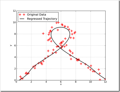
Lets start with a picture. This graph shows a trajectory fit to noisy data. Measurements on the trajectory are shown as red crosses and the regressed trajectory is shown as the black line. By the last entry of this tutorial, solving this kind of problem will be easy with a few lines of python.
The Basics – Linear Regression using Polynomials
The usual regression question is how to fit a polynomial to a set of data. There is more to this question than appears at first. Fitting data involves answering the question of what is ‘best’. Linear regression answers that question by providing an answer that minimizes the sum if squares of difference between the fit and the data. This answer is useful in many cases, but not always! There are other answers.When fitting data to a polynomial, regression minimizes this expression:

In this expression, xi and yi, are a data tuple and wi is the weighting to apply to each power of xi . The wi values are selected to minimize the squared difference between the estimate, which is a function of x, and the measurement y. This expression is used because it is easy to solve (once you know how), and it describes the maximum likelihood answer if the polynomial describes the relations between x and y (e.g. if there were no errors, the equations perfectly describe what is happening), the measurement errors are not correlated (e.g. independent and identically distributed – iid) and the errors have a zero mean gaussian distribution. Even when this is not the case, this approach is pretty good.
This equation can be solved in many ways with readily available software packages. In the Numpy libraries there is polyfit. Numpy also has lstsq, which solves a least squares fit. Argonne National Labs has a least squares fit package here that can find the best polynomial (or other families of functions). For this tutorial, things will be solved the hard way before existing libraries are used.
If the value for y are formed into a vector, and a special matrix, known as the Vandermonde matrix, is formed from the values of x, then the result is a linear system of equations.
 This matrix can be formed using the vander function in Numpy.For a fitting problem is in this form, it can be neatly expressed using matrix notation.
 This can be solved numerically using an optimizer in scipy like fmin_slqp. This can be a very computationally expensive way to solve the problem (e.g. it takes a long time to solve). A more computationally efficiency (e.g. faster) way to solve this problem is to use the KKT conditions. This not only works, but results in the global optimum, because this problem is convex. This is important, because not all problems can easily be solved for the global optimum. Some problems have many local optimums, which make it difficult to find the best overall answer. Using the KKT conditions, the optimum values for w* are found using simple matrix operations.
A first example, the hard way…
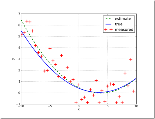
Before fitting a curve to data, it helps to have data. The following python script will data for a quadratic relationship between x and y. The measurements of y will be corrupted by a Gaussian (or normal) noise. This model is expressed aswith the random noise described by
This python script will build a useful data set.
from pylab import *
from random import normalvariate

a = 0.03
b = –0.21
c = 0.4
f = lambda x,a=a,b=b,c=c:a*x**2+b*x+c
xList = arange(-10,10,0.25)
yListTrue = [f(x) for x in xList]
yListMeasured = [y+normalvariate(0,1) for y in yListTrue]
This script takes the lists of points and finds the best quadratic fit for the data.
# fit the data
def polyFit(xList,yList,order=1):
    '''fit the data using a least squares and polynomial'''
    fList = [(lambda x,n=n: x**n) for n in range(order,-1,-1)]
    # build row for each element in y
    bList = []
    A_List = []
    for (thisX,thisY) in zip(xList,yList):
        bList.append(thisY)
        A_Row = [f(thisX) for f in fList]
        A_List.append(A_Row)
    b = matrix(bList).T
    A = matrix(A_List)
    w = inv(A.T*A)*A.T*b
    return w.T.tolist()[0]

w = polyFit(xList,yListMeasured,order=2)
aHat = w[0]
bHat = w[1]
cHat = w[2]

# summarize the results
print 'Data model is   :%4.2f*x^2 + %4.2f*x + %4.2f' % (a,b,c)
print 'Fit equation is :%4.2f*x^2 + %4.2f*x + %4.2f' % (aHat,bHat,cHat)

# plot, for visual comparison
def getPolyF(w):
    '''create a function using the fit values'''
    return lambda x,w=w: sum([thisW*(x**(len(w)-n-1))
                            for n,thisW in enumerate(w)])

fHat = getPolyF(w)
xPlotList = arange(-10,10,0.1)
yEstList = [fHat(x) for x in xPlotList]
fTrue = getPolyF([a,b,c])
yTrueList = [fTrue(x) for x in xPlotList]

figure(1)
plot(xPlotList,yEstList,'--g',linewidth=2)
plot(xPlotList,yTrueList,'b',linewidth=2)
plot(xList,yListMeasured,'+r',markersize = 12,markeredgewidth=2)
xlabel('x')
ylabel('y')
legend(['estimate','true','measured'])
grid(True)
savefig('secondOrderFitEx.png')
show()
When this script is run, the console output isDifferent answers will occurs on each run because random numbers are used.Data model is :0.03*x^2 + -0.21*x + 0.40 Fit equation is :0.03*x^2 + -0.26*x + 0.46

Another example, simpler this time…
In the first example, a lot of the code was built by hand. To make the task easier, the libraries in Numpy & Scipy are used.The first change is to incorporate the vander function and psuedo inverse, pinv, functions into the polyFit function. The vander function builds the Vendermonde matrix and the pinv function performs the same operation as inv(A.T*A)*A.T
def polyFit(xList,yList,order=1):
    '''fit the data using a least squares and polynomial'''
    A = vander(xList,order+1)
    b = matrix(yList).T
    w = pinv(A)*b
    return w.T.tolist()[0]
Alternatively, the polyFit function could be created using the lstsq function. This function is nice because it provides additional information that can be useful in checking on the quality of a fit.def polyFit(xList,yList,order=1):
'''fit the data using a least squares and polynomial'''
A = vander(xList,order+1)
b = matrix(yList).T
(w,residuals,rank,sing_vals) = lstsq(A,b)
return w.T.tolist()[0]Finally, the polyFit function could be eliminated entirely, and replaced with the polyfit function. The second change is to replace the getPolyF function with the poly1d function in Numpy. This gets rid of a few lines of code.
fHat = poly1d((aHat,bHat,cHat))
xPlotList = arange(-10,10,0.1)
yEstList = [fHat(x) for x in xPlotList]
fTrue = poly1d((a,b,c))
yTrueList = [fTrue(x) for x in xPlotList]
Combining all of these changes, the example script becomes….
from pylab import *
from random import normalvariate

# generate the data
a = 0.03
b = -0.21
c = 0.4
f = lambda x,a=a,b=b,c=c:a*x**2+b*x+c
xList = arange(-10,10,0.5)
yListTrue = [f(x) for x in xList]
yListMeasured = [y+normalvariate(0,1) for y in yListTrue]

# fit the data
w = polyfit(xList,yListMeasured,2)
aHat = w[0]
bHat = w[1]
cHat = w[2]

# summarize the results
print 'Data model is   :%4.2f*x^2 + %4.2f*x + %4.2f' % (a,b,c)
print 'Fit equation is :%4.2f*x^2 + %4.2f*x + %4.2f' % (aHat,bHat,cHat)

# plot, for visual comparison
fHat = poly1d((aHat,bHat,cHat))
xPlotList = arange(-10,10,0.1)
yEstList = [fHat(x) for x in xPlotList]
fTrue = poly1d((a,b,c))
yTrueList = [fTrue(x) for x in xPlotList]

figure(1)
plot(xPlotList,yEstList,'--g',linewidth=2)
plot(xPlotList,yTrueList,'b',linewidth=2)
plot(xList,yListMeasured,'+r',markersize = 12,markeredgewidth=2)
xlabel('x')
ylabel('y')
legend(['estimate','true','measured'])
grid(True)
savefig('secondOrderFitEx.png')
show()
The real work for fitting the polynomial is now done by one line of code, and the reconstruction of the curve is done by another.The reason for performing the fits using custom code is so later, more interesting fits can be found.
See part 2 for a tutorial on weighted fitting & regression.
All text is copyright © 2010, Ed Tate, All Rights Reserved.
All software and example codes are subject to the MIT License
Copyright (c) 2010, Ed Tate, Permission is hereby granted, free of charge, to any person obtaining a copy of this software and associated documentation files (the "Software"), to deal in the Software without restriction, including without limitation the rights to use, copy, modify, merge, publish, distribute, sublicense, and/or sell copies of the Software, and to permit persons to whom the Software is furnished to do so, subject to the following conditions: The above copyright notice and this permission notice shall be included in all copies or substantial portions of the Software.
THE SOFTWARE IS PROVIDED "AS IS", WITHOUT WARRANTY OF ANY KIND, EXPRESS OR IMPLIED, INCLUDING BUT NOT LIMITED TO THE WARRANTIES OF MERCHANTABILITY, FITNESS FOR A PARTICULAR PURPOSE AND NONINFRINGEMENT. IN NO EVENT SHALL THE AUTHORS OR COPYRIGHT HOLDERS BE LIABLE FOR ANY CLAIM, DAMAGES OR OTHER LIABILITY, WHETHER IN AN ACTION OF CONTRACT, TORT OR OTHERWISE, ARISING FROM, OUT OF OR IN CONNECTION WITH THE SOFTWARE OR THE USE OR OTHER DEALINGS IN THE SOFTWARE.


